Uncertainties in Measurement
Kreshnik Angoni
BRIEF SURVEY OF UNCERTAINTY IN PHYSICS LABS
FIRST STEP: VERIFYING THE VALIDITY OF RECORDED DATA
The drawing of graphs during lab measurements is a practical way to estimate quickly:
a) Whether the measurements confirm the expected behaviour predicted by the theory
b) If any of recorded data is measured in a wrong way and must be excluded from further data
treatments.
Example:
We drop an object from a window and, from free fall model calculations, we expect it to hit ground after 2sec. To verify our
prediction, we measure this time several times and record the following results:
1.99s, 2.01s, 1.89s, 2.05s 1.96s, 1.99s, 2.68s, 1.97s, 2.03s, 1.95s
- (Note: 3-5 measurements is a minimum acceptable number of data for estimating a parameter during a lab session, i.e. repeat the measurement 3-5 times)
- (Note: 3-5 measurements is a minimum acceptable number of data for estimating a parameter during a lab session, i.e. repeat the measurement 3-5 times)
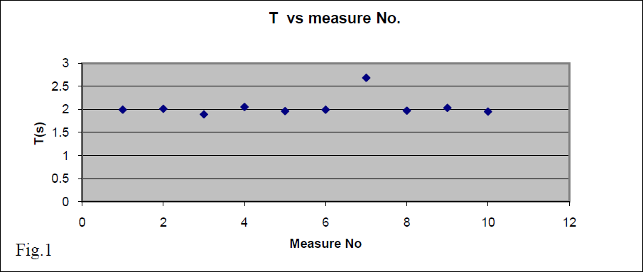
To check out those data we include them in a graph (fig.1). From this graph we can see that:
a) The falling time seems to be constant and very likely ~2s. So, in general, we have acceptable data.
b) The seventh measure seems too far from the others results and this might be due to an abnormal circumstance during its measurement. To eliminate any doubt, we exclude this value from the following data analysis. We have enough other data to work with. Our remaining data are:
1.99s, 2.01s, 1.89s, 2.05s, 1.96s, 1.99s, 1.97s, 2.03s, 1.95s.
SECOND STEP: ORGANIZING RECORDED DATA IN A TABLE
Include all data in a table organized in such a way that some cells be ready to include the uncertainty
calculation results. In our example, we are looking to estimate a single parameter “T”, so we have to
predict (at least) two cells for its average and its absolute uncertainty.
Table 1
| T1 | T2 | T3 | T4 | T5 | T6 | T7 | T8 | T9 | Tav | ΔT |
| 1.99s | 2.01s | 1.89s | 2.05s | 1.96s | 1.99s | 1.97s | 2.03s | 1.95s |
THIRD STEP: CALCULATIONS OF UNCERTAINTIES
The true value of measured parameter is unknown. We use the recorded data to find an estimation of the true value and the uncertainty of this estimation.
Three particular situations for uncertainty estimations
A] - We measure a parameter several times and always get the same numerical value.
Example:
We measure the length of a table three times and we get L= 85cm and
a little bit more or less.
This happens because the smallest unit of the meter stick is 1cm and we cannot be precise about what portion of 1cm is the quantity “a little bit more or little bit less”.
In such situations we use “the half-scale rule” i.e.; the uncertainty is equal to the half of the smallest unit available for measurement.
In our example ΔL= ±0.5cm and the result of measurement is reported as L= (85.0 ± 0.5)cm.
-If we use a meter stick with smallest unit available 1mm, we are going to have a more precise result but even in this case there is an uncertainty.
Suppose that we get always the length L= 853mm.
Being aware that there is always a parallax error (eye position) on both sides reading, one may get ΔL= ± 1, 2mm (and even 3mm, ) depending on the measurement circumstances.
In this situation, it is suggested to accept 1 or 2 units of measurement.
The result is reported L= (853 ± 1)mm .
Our estimation for the table length is 853mm. Also, our measurements show that the true length is between 852 and 854mm.
The uncertainty interval is (852, 854)mm.
The absolute uncertainty of estimation is ΔL= ± 1mm
-Now, suppose that, using the same meter stick, we measure the length of a calculator and a room and find Lcalc= (14.0 ±0.5)cm and Lroom= (525.0 ±0.5)cm.
In the two cases we have the same absolute uncertainty ΔL= ± 0.5 cm, but we are conscious that the length of room is measured more precisely.
The precision of a measurement is estimated by the uncertainty portion that belongs to the unit of measured parameter. Actually, it is estimated by the relative error:
.
-Smaller relative error means higher precision of measurement. In our length measurement, we have:
We see that the room length is measured much more precisely (about 38 times).
Note: Don't mix the precision with accuracy! A measurement is accurate if the uncertainty interval contains an expected (known) value and non-accurate if it does not contain it.
B] - We measure a parameter several times and always get different numerical values.
Example:
We drop an object from a window and we measure the time it takes to hit ground. We find the different values of time intervals inserted in table _1. In cases like this, we have to calculate the average value and the absolute uncertainty based on statistical methods.
B.1) We estimate the value of parameter by the average of measured data.
In case of our example:
B.2) To estimate how far from the average can be the true value we use the spread of measured data.
A first way to estimate the spread is by use of mean deviation i.e. “average distance” of data from their average value. In case of our example we get:
Now we can say that the real value of fall time is inside the uncertainty interval (1.947, 2.017)s or between = 2.017s and = 1.947s with average value 1.982s.
Taking in account the rules of significant figures and rounding off:
- The result is reported as T = (1.98 +/- 0.04)s
- The result is reported as T = (1.98 +/- 0.04)s
Another (statistically better) estimation of spread is the standard deviation of data.
Based on data for falling time (T) in our first example and the mathematical expression for the standard deviation we get:
The result is reported as T = (1.98 +/- 0.05)s
B.3) For spread estimation, the standard deviation is a better estimation for the absolute uncertainty.
This is because a larger interval of uncertainty means a more “conservative estimation” but in the same time a more reliable estimation.
Note that we get ΔT= +/- 0.05 s when using the standard deviation and ΔT= +/- 0.03 s when using the mean deviation. Also, the relative error (relative uncertainty) calculated from the standard deviation is bigger. In our example, the relative uncertainty of measurements is:
(when using the standard deviation)
(when using the mean deviation)
Note: We will accept that our measurement is enough precise if the relative uncertainty “” is smaller than 10%.
If the relative uncertainty is > 10%, we may proceed by:
- Cancelling the data “shifted the most from the average value”
- Increasing the number of data by repeating more times the measurement
- Improving the measurement procedure
C] - Estimation of uncertainties for calculated quantities (uncertainty propagation).
Very often, we use the experimental data recorded for some parameters and a mathematical expression to estimate the value of a given parameter of interests (POI). As we estimate the measured parameters with an uncertainty, it is clear that the estimation of POI will have some uncertainty, too. Actually, the calculation of POI average is based on the averages of measured parameters and the formula that relates POI with measured parameters. Meanwhile, the uncertainty of POI estimation is calculated by using the Max-Min method. This method calculates the limits of uncertainty interval, and by using the formula relating POI with other parameters and the combination of their limit values in such a way that the result be the smallest or the largest possible.
Example:
To find the volume of a rectangular pool with constant depth , we measure its length, its width and its depth and then, we calculate the volume by using the formula V=L*W*D.
Assume that our measurement results are L = (25.5 ± 0.5)m, W = (12.0 ±0.5)m, D = (3.5 ±0.5)m.
In this case, the average estimation for the volume is .
This estimation of volume is associated by an uncertainty calculated by Max-Min method as follows:
So, the uncertainty interval for volume is (862.5, 1300.0) and the absolute uncertainty is:
while the relative error is:
Note: When applying the Max-Min method to calculate the uncertainty, one must pay attention to the mathematical expression that relates POI to measured parameters.
Example:
-You measure the period of an oscillation and you use it to calculate the frequency (POI).
As , ,
the Max-Min method gives
and .
- If , then
and and .
Note_2: Another way to calculate is by use of the formula
after finding the limits of its uncertainty interval.
The standard deviation can be calculated direct in Excel and in many calculators
HOW TO PRESENT THE RESULT OF UNCERTAINTY CALCULATIONS
You must provide the average, the absolute uncertainty and the relative uncertainty. So, for the last example, the result of uncertainty calculations should be presented as follows:
, .
Note: Uncertainties must be quoted to the same number of decimal digits as the average value. The use of [scientific notation] helps to prevent confusion about the number of significant figures.
Example:
If calculations generate, say A = (0.03456789 ± 0.00245678). This should be presented after being rounded off (leave 1,2 or at maximum 3 digits after decimal point):
or
HOW TO CHECK IF TWO QUANTITIES ARE EQUAL
This question appears essentially in two situations:
- We measure the same parameter by two different methods and want to verify if the results are equal.
- We use measurements to verify if a theoretical expression is right.
In the first case, we have to compare the estimations and of the “two parameters”. The second case can be transformed easily to the first case by noting the left side of expression A and the right side of expression B. Then, the procedure is the same.
Example:
We want to verify if the thins lens equation is right. For this we note and .
Rule: We will consider that the quantities A and B are equal if their uncertainty intervals overlap.
They should be in the same units.
WORKING WITH GRAPHS
We may use graphs to check the theoretical expressions or to find the values of physical quantities.
Example:
We find theoretically that the oscillation period of a simple pendulum is and we want to verify it experimentally.
For this, as a first step, we prefer to get a linear relationship between two quantities we can measure; in our case period T and length L. So, we square both sides of the relationship and get:
Next, after noting and we get the linear expression
Y = a*X where .
So, we have to verify experimentally if there is such a relation between and L.
Note that, if this expression is confirmed, we may use the experimental value of a to calculate an estimation for the free fall constant g by expression:
“”.
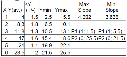
Assume that, after measuring several times the period for a given pendulum length, one calculates the average value and uncertainty for y(=T^2). By repeating this procedure for different values of length x(L=1,..,6m) one get the data shown in table No 1.
Table 1

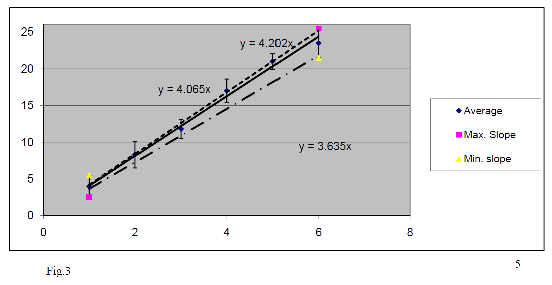
At first, we graph the average data. We see that they are aligned on a straight line; this confirms the theoretic expression, as expected. Next, we use Excel to find the best linear fitting for our data and we request to this line to pass from (X = 0, Y = 0) because this is predicted from the theoretical formula.
We get a straight line with:
.
Using our theoretical formula we calculate the estimation for
which is not far from expected value 9.8.
Next, we add the uncertainties in the graph and draw the best linear fitting with maximum /minimum slope that pass by origin.
From these graphs we get:
and
.
So, we get:
and
.
This way, by using the graphs we:
- proved experimentally that our theoretical relation between T and L is right.
- found that our measurements are accurate because the uncertainty interval (9.38, 10.85) for “g” does include the officially accepted value
- found the absolute error Δg =
The relative error is ε = (0.735/9.70)*100% = 7.6% which means an acceptable (ε < 10%) precision of measurement.
ABOUT THE ACCURACY AND PRECISION
- Understanding accuracy and precision by use of hits distribution in a Dart’s play.
-The estimation of accuracy is essential during a calibration procedure. As a rule, before using a method (or device) for measurements, one should make sure by measurements that it does produce accurate results in the range of expected values for the parameter under study. During such a procedure one knows in advance the “officially accepted value” which is expected to be the measurement result.
If the result of measurement is unknown previously, there is no sense to talk about the accuracy. Meanwhile, during any kind of measurement one must report the relative uncertainty i.e. the precision of measurement .
-So, we will refer to accuracy only in those labs that deal with an officially accepted value for a given parameter like free fall acceleration "g", Planck constant "h", etc. In principle, there is an accurate experiment result if the “average of data” fits to the” officially accepted value”.
We will consider that our experiment is “enough accurate” if the ” officially accepted value” falls inside the interval of uncertainty for the estimated parameter; otherwise we will say that the result is inaccurate.


