Motion Along a Straight Line: Graphical Representation
Helena Dedic
x-t graphs
Average velocity from the x - t graph
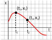
The slope of the secant line is equal to the average velocity during an interval of time .
To determine the average velocity we find the two points on the curve corresponding to instants of time and .
Then we determine the "coordinates" of these points and then we are ready to compute the average velocity:
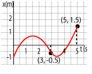
For example, we want to determine the average velocity during the last two seconds of motion of a particle. Its motion is illustrated by a graph below:
Therefore the average velocity is:
Instantaneous velocity from the x - t graph
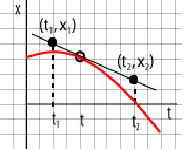
The slope of a tangent line drawn at a point (x,t) is equal to the instantaneous velocity at t.
To determine the instantaneous velocity we first draw a tangent line at (x,t).
Then we choose two points on the tangent line and then determine the "coordinates" of these two points. We can then compute the instantaneous velocity:
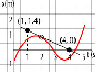
For example, we want to determine the velocity at 2 s of a particle. Its motion is illustrated by a graph below:
We draw the tangent line at (2, 0.9). Then we choose two points on the tangent line. In this case, we chose the points (1, 1.4) and (4, 0). Then we compute:
v - t graph from x - t graph
When sketching a v - t graph we follow these steps:
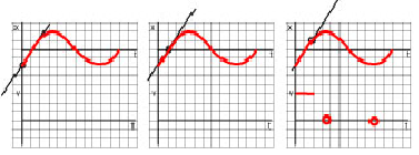
1. Move a ruler along the curve from left to right so that it shows the tangent line. Note when the ruler is horizontal, that is when the slope of the tangent line is zero.
For each such instance record the instant (or interval of) time on t-axis of the v - t graph. The v - t graph will cross t-axis at those points. The graphs below show the movement of the "ruler" until it reaches the first point of zero velocity.

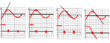
2. Move the ruler again along the curve from left to right so that it shows the tangent line. Note the intervals of time when the ruler does not change its slope.
For each such instance note whether the slope is positive or negative. Then draw for each such interval a horizontal line on the v - t graph. The horizontal line should be above t-axis when the slope is positive and below t-axis when the slope is negative. The graphs below show the movement of the "ruler" along a straight line segment of the x - t graph. Note that the "ruler" does not change its slope.
3. Move the ruler again along the curve from left to right so that it shows the tangent line. Note the intervals of time when the ruler turns while moving along the curve. It indicates that the slope of the x - t graph is changing.
When the ruler turns clockwise then the slope of the x - t graph is decreasing and when the ruler turns counterclockwise then the slope of the x - t graph is increasing. For each such instance draw a straight line with a negative slope (clockwise) or positive slope (counterclockwise) on the v - t graph. The graphs below show the movement of the "ruler" along a curved line segment of the x - t graph. Note that the "ruler" does changes its slope from positive to negative and that it rotates clockwise. The incomplete v - t graph shows decreasing velocity.
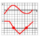
4. It is important to say that the resulting graph should be continuous and that any discrepancy that you encounter when drawing the graph are due to some error somewhere. Check your work.
The complete v - t graph looks like this:
Understanding v-t Graphs
Table of Synonyms
Note that the following sketches are examples of motion and cannot be generalized.
| Synonymous statements | v-t graph |
|---|---|
|
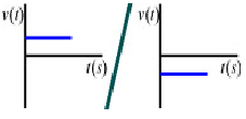
The velocity graph is above or below t - axis |
|
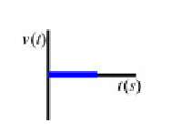
The graph runs along t-axis. |
|
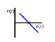
The graph of velocity vs. time crosses the t-axis - see the dot in the graph. |
|
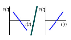
The velocity graph has a negative/positive slope |
|
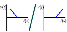
The velocity graph "approaches" the t-axis in the two graph on the left (slowing down). The velocity graph "goes away" from t-axis in the two graph on the right (speeding up).
|
Important Points to Remember
- The instantaneous acceleration is the slope of the v - t graph.
- A straight line v - t graph indicates motion with constant acceleration.
- A straight and horizontal v - t graph indicates motion with zero acceleration.
- Important notions:
- v = 0 does not imply that a = 0
- a = 0 implies that v is constant
- "speeding up" implies only that the acceleration and the velocity have the same direction while "slowing down" implies that they have the opposite direction
- The speed is equal to the absolute value of the velocity. When thinking about speed visualize a graph of absolute value of velocity versus t
Relationship between x-t and v-t graphs
How to compute the displacement from the v-t graph
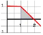
The area under the graph tells us about the displacement during an interval of time Dt = t2 - t1. When we say "area under the graph" we mean an area bound by the segment of the t-axis (t1, t2), by the segment of the vertical line drawn from point t1 on the axis to the corresponding point on the curve, by another segment of the vertical line drawn from point t2 on the axis to the corresponding point on the curve and by the segment of the curve (v(t1, v(t2)). It is important to note that the displacement is positive if the area is above the t-axis and negative if it is below the t-axis. For example, the displacement during the interval of time (1 s,2 s) is equal to the shaded area shown below. The blue lines indicate the boundaries of this area.
The area of this triangle is equal to ½x1 m/s x1 s = 0.5 m. Note that we have only found the displacement during this interval of time. To determine the position of the particle at the end of this interval of time, we have to add the displacement to the position of the particle at the beginning of the interval of time. Let say that the position of the particle was 0 at t = 0. During the first second of motion the particle traveled 1 m and therefore at the beginning of the interval of time we dealt with the position was 1 m. The position at t = 2 s is the sum of the initial position and the displacement or 1 + 0.5 = 1.5 m. Similarly, the displacement during the interval of time (3 s, 4 s) is shown by the shaded area in the graph below.
In this case, the area is below the t-axis and so the displacement is equal to -1 m/s x 1 s = - 1 m. To find the position at 4 s, we would have to add - 1 m to the position at 3 s.
Exercises
Simulations
Qi Luo


