Measurement and Data Analysis

Kreshnik Angoni

ABOUT PHYSICS

Physics is one of the natural sciences; so it deals with the two nature components: matter and fields.

The object of physics is the study of motion in nature:

“HOW does evoluate and WHY a given MOVEMENT(of matter or field) is produced”.

How does the study of physics proceed? It starts by defining the objective (say-study of a soccer ballmotion) and the reference frame where the motion is studied (say- field sides).

Next, one follows by identifying the necessary parameters for description of the movement (example; position, velocity, acceleration).
Next, one records a set of data for each parameter.
Then, one looks for any possible relationship pattern between the measured data. The easiest way to do this is by using a graph.

Next, if a graphical pattern appears, one tries to get a mathematical expression for the relation between the parameters in graph.

Then, one builds a theoretical model to explain the observed relationship and gets one (or several) equation that relates the considered parameters.

After that, one uses the model and its equations to predict the numerical values of these parameters in any similar situation (experiment).

Example: Object of study: The motion of a glider on an air track (select track as reference frame).

Parameters : velocity and time.

Measurement:

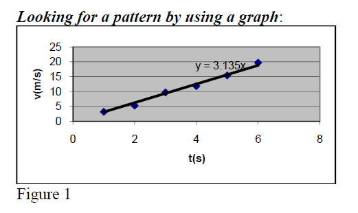
Getting a mathematical relation from the graph

Build a graph with recorded data. Find out a linear relationship

v(m/sec) = 3.1352*t(sec)

Building a model:

One considers that the glider can be modeled by a material point with mass = mgl and considers the movement of material point with constant acceleration a = v/t.

Result: The glider moves as a material point with acceleration $a=3.1352m/s^{2}\,\!$.

UNITS

A physical parameter is characterised by a numerical value and a unit of measurement.

In physics, one discerns the basic units and the derived units.

a) A basic unit is a unit used during a direct measurement. In this case the numerical value of the physical parameter is equal to the number of times the basic units enters into the parameter in consideration.

(Example: When measuring the length of a table, one has to define first what unit will use - say meter. Then it verifies haw many times the meter unit enters into the length of the table - say1.6 times. So, one gets that the table length is 1.6meters.)

The basic units are selected following the humanity experience and fit well with a wide range of measurements.

The basic unit of the physical parameter “length” is the meter (m).

The universal etalon of meter, kept in Sevres (France), is defined as the distance between two fine scratches on a special material bar. All meter units used over the world must be equal to this etalon.

The basic unit of the physical parameter ”time” is the second (s) and it is the time light takes to travel over 299 792 458m(~3*106m/s) in vacuum.

All second units used over the world have to be equal to this etalon.

The basic unit of physical parameter “mass” is the kilogram (kg) and it is defined as the mass of a particular metal cylinder kept in Sevres.

All kilogram units used over the world have to be equal to this etalon.

The meter, the sec. and kg are the basic units in SI (Système International) system of units.

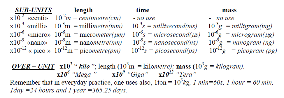
Although the etalons are selected to produce logical numerical values for everyday measurements, the continuous increase of human activity requires dealing with numerical values, which are pretty big or small if referred in basic units. To avoid this problematic, one introduced subsequent definitions:

- For historical reasons there are several different units used for the same physical quantity. For example the distance is expressed in miles (mi) or inches (in), too.

(Example: One may see the speed given in Km/hr and miles/hr in some cars).

How to find the value of a physical propriety in a given unit when we know its value in another unit? This question is answered by the procedure of unit conversions (see next sections).

Example: We know that the distance between two cities is 425km and we wants to find it in miles.

From the manual we find that 1 mi =1.609Km. So, 1 km = (1/1.609) mi and (1mi/1.609km)=1.

We multiple our expression by 425 km*1= 425km*(1mi/1.609km) = 264.14 mi.

b) A derived unit is a unit that is expressed through the basic units.

Example: the volume is expressed in $m^{3}$; the density of a liquid is expressed in kg/$m^{3}$.
There are three basic units (in SI system m, sec, kg) and many derived units ($m^{2}$, $m^{3}$, N, m/s, $m/s^{2}$…)

DIMENSIONAL ANALYSIS

- In physics, one uses often expressions of type ” this parameter has length dimensions”. So, without being interested on the real unit (meter, mile, cm ) one confirms that the parameter is expressed in length units. The three basic dimensions are “L for length”, “T for time” and “M for mass”.

When referring to the dimension of a given physical quantity one uses the square brackets.

Ex.: [a] = $LT^{-2}\,\!$ for the dimension of acceleration.

Suppose that calculations produce an algebraic expression for the required physical quantity. As a first step of verification, one may use the dimensional analysis. So, if the expression is Z = X + A, at first, one has to verify that [X] and [A] are equal because one can not add up different physical quantities (Ex. position + acceleration!!) So, before proceeding to numerical calculations, one must verify the dimensional consistency of the found expression to the dimension of required quantity.

Ex.: If a calculation gives for acceleration the expression a = ${\frac {m*t^{2}}{v}}\,\!$, by verifying the dimensions;

[a] = ${\frac {[m]*[t^{2}]}{[v]}}={\frac {M*T^{2}}{L/T}}=M*T^{3}*L^{-1}\,\!$

it is a wrong expression because [a] = $LT^{-2}\,\!$.

CONVERSION OF UNITS

Often, one needs often to convert the result ( for a physical quantity) from a given unit to another unit.

“How to convert the value of a physical propriety from a given unit to another unit”?
To do this one has to use the conversion procedures.

At first, one refers to conversion factors; Ex: 1 h = 60 min; 1 h = 3600 s; 1mi = 1.609km

The ratio of all conversions is equal to 1; (1h/60min) =1 (1h/3600s) = 1; (1mi/1.609km) =1.

Then, as the multiplication by 1 does not change the result one goes step by step ;

Ex 1: The distance between two cities is 425km and we want to find it in miles. From the manual we find that 1 mi =1.609Km

So, ${\frac {1mi}{1.609km}}=1$ and so:

$425km=425*{\frac {1mi}{1.609km}}=264.4mi$ 

Ex 2: Convert the speed 60km/h in m/s. As 1km = 1000m, 1000m/1km =1 and 1h/3600s =1,

60km/h = $60*{\frac {1000m}{1km}}*{\frac {1h}{3600s}}\,\!$ = 16.67 m/s 

Ex 3: The area of a paper sheet is $6580cm^{2}$. Convert it in $m^{2}$. Knowing that 1 m = 100cm and

$6580cm^{2}=6580cm*cm=6580cm*({\frac {1m}{100cm}})*cm*({\frac {1m}{100cm}})=6580({\frac {1}{100}})m({\frac {1}{100}})m=0.658m^{2}\,\!$ 

Ex 4:

Area = $1in^{2}=[1in*({\frac {2.54cm}{1in}})*({\frac {1m}{100cm}})]^{2}=[2.54m/100]^{2}=[2.54*10^{-2}m]^{2}=6.4516*10^{-4}m^{2}$

Vol = 1 litre(l) = $10cm*10cm*10cm=10^{3}cm^{3}=10^{3}({\frac {1}{100m}})^{3}=10^{3}(10^{-2}m)^{3}=10^{3}*10^{-6}m^{3}=10^{-3}m^{3}$ 

SCIENTIFIC NOTATION

Although the units are selected to produce “normal values” for physical quantities, the practice shows that often one has to deal with very big or very small values of a physical quantity.

In these situations the use of scientific notation avoids errors and simplifies the calculations.

When written in scientific notation, the numerical value of considered quantity is presented as a number with one digit before the decimal point multiplied by a factor of 10. (Ex. $1.253x10^{-8}\,\!$; $-8.253x10^{-38}\,\!$).

The scientific notation of a number is known also as its exponential presentation with base 10.

To convert a number to scientific notation move the decimal point to the right or the left until you get one digit on the left of decimal point.

To keep the same number value, for each left shift multiply by 10 and for each right shift divide by 10.

Ex1:

$125.4=125.4*10^{0}=12.54*10^{1}=1.254*10^{2}\,\!$ 

$0.001254=0.001254*10^{0}=0.01254*10^{-1}=0.1254*10^{-2}=1.254*10^{-3}\,\!$ 

Basic operations with scientific numbers. Given two numbers:
$x_{0}=a_{0}10^{b_{0}}$, $x_{1}=a_{1}10^{b_{1}}$

$x_{0}*x_{1}=(a_{0}a_{1})*10^{b_{0}+b_{1}}$ and ${\frac {x_{0}}{x_{1}}}=({\frac {a_{0}}{a_{1}}})*10^{b_{0}-b_{1}}\,\!$ 

Ex2:

$(5.67*10^{-5})*(2.34*10^{2})=13.2678*10^{-3}=1.32678*10^{-2};(5.67*10^{-5})/(2.34*10^{2})=2.423*10^{-7}\,\!$ 

Before performing addition or subtraction the numbers must be presented by the same exponent.

Usually the smaller number is transformed before performing the addition or subtraction.

Ex3:

$3.17*10^{-5}+1.34*10^{-4}=0.317*10^{-4}+1.34*10^{-4}=1.657*10^{-4}\,\!$ 

$2.13*10^{6}-5.34*10^{2}=2.13*10^{6}-0.000534*10^{6}=2.130534*10^{6}\,\!$ ≅ $2.13*10^{6}\,\!$

SIGNIFICANT FIGURES

In experimental measurements, one has to deal with a “minimal available unit” and this defines the uncertainty of the measurement.

For example, when measuring the length of an object by using a ruler with minimum unit scale 1mm,
 
if you report the result of measurement L = 17.5mm, it means that the its length is estimated
 
with three significant figures and the last digit “5” is uncertain. 

The concept of significant figure(reliable digit) is related to measurable parameters.

If the length is reported as 12.345 m, then this is a number with 5 significant figures
 
where last figure “5” is not certain. 

From the practical point of view, this means that in that measurement the minimum unit was 0.01m = 1cm and it is accepted that the observer is able to distinguish without being sure a length 0.5 cm.

In majority of cases, by convention, during a measurement process, one assumes that the uncertainty

of measured value is 0.5 of minimum available unit.

In the above example the uncertainty is 0.5mm and the true length value is inside the interval (17.5 ± 0.5) mm.

Note: If the mass of an object is reported 15.5g, the uncertainty is 0.5g but if reported 15.55g, it is 0.05g.

• Considering a data treatment situation, one has to remember that the number of digits at absolute

uncertainty (or absolute error) defines the number of digits at reported values.

Ex: One uses a meter stick with 1 cm unit (Δ = 0.5cm) to measure the length of a set of wood beams and gets values 17.5, 18.5, 18.5….

[Absolute uncertainty is 0.5cm (or smaller, i.e. 0.2cm or 0.1cm depending on observer ability)]

Then, one calculates the average length of the set and gets the average value 18.311cm.

As the absolute uncertainty is Δ= ±0.5cm, there is no sense to keep more than one digit after decimal point at the average.

The second and the third digits after the decimal point of average value have no reliability because they are much smaller that accepted value for the uncertainty.

So, one must round off the number to one decimal digit and the average length of the set must be reported as (18.3± 0.5)cm.

How to find the number of significant figures:

1. All nonzero digits are significant: 1.324 g has 4 sign. fig., 1.5 g has 2 sign. figures.


2. Zeroes between nonzero digits are significant: 3002 kg has 4 sign. fig.; 1.02 L has 3 sign. figures.


3. Leading zeros to the left of the first nonzero digits are not significant; 0.001g has 1 sign. figure; 0.012 g has 2 sign.figures. Such zeroes merely indicate place holders and they do not contain any information about the uncertainty of estimated parameter.
   Often one uses the scientific notation to obtain quickly the sig. figure.
   Ex: $0.0001035=1.035*10^{-}5\,\!$ (4 sign.fig)


4. Trailing zeroes (to the right end) are significant only if there is a decimal point.
   0.0230 m has 3 sign. figures. 0.20 g has 2 sign. figures.
   but $100=1*10^{2}\,\!$ has 1 sig.figure.
   while $100.0=1.000*10^{2}$ has 4 sign. figures.


5. In scientific notation the significant figures are counted at the coefficient.
   Ex. The length 5.5mm has 2 sig. figures even if converted in meters;
   It is 0.0055m which is written $5.5*10^{-3}$ m(2 sig. figure).
   $2.02*10^{4}$ kg has 3 sign. figures,
   $2.020*10^{4}$ ft has 4 sign.figures
   and $2.0200*10^{4}$ N has 5 sign. figures.


6. In addition and subtraction, the result is rounded off to the smallest number
   of decimal places occurring in all components.
   200(no decimals) + 25.643 (5 sign. figures) = 225.643
   which should be rounded off to 226 (no decimals).
   
   In multiplication and division, the result should be rounded off
   so as to have the same number of significant figures as in the component
   with the smallest number of significant figures.
   
   4.0 (2 sign. figures) × 13.60 (4 sign. figures) = 54.400
   which should be rounded off to 54 (2 sign. figures).
   
   12.589(5 sign. figures) x 2.0312(5 sign. figures) / 4.0 (2 sign. figures) = 6.3926942
   which should be rounded off to 6.4 (2 sign. figures).


7. Rounding off rules: When rounding off, use only the first number to the right
   of the assumed uncertain digit(ignore the following digits)
   
   Example:
   
   For two significant figures, 18.71 is rounded to 19 and 18.46 to 18.
   Similarly, 5.249 is rounded to 5.2 not 5.3;
   18.51 is rounded to 19 (if the digit to be dropped is 5
   followed by a 0 digit leave it as it is, otherwise increase it by 1)

Basic principle in numerical calculations:

The result cannot be more precise than parameters included in calculations.

Step-by-step procedure:

1. Identify the sig.figures and number of decimals for each number before calculations.


2. Identify the smallest sig.fig in multipl./div. and smallest number of decimals in substr./add.


3. Do first the mathematical calculations in normal mathematical way; get a mathematical result.


4. At the end, round off the found mathematical result by referring to:
   

   a) The smallest number of digits after decimal point for substraction /addition
   

   b) The smallest sig.fig. for division/multiplication
   

Ex: 124.4 + 2.345 –11.005 = 115.74 and by rounding of (to 1 digit after dec. point) we get 115.7 (5.345 +12.3005) / 2.2 = 8.02068 and by rounding off (to 2 sig.fig) we get 8.0 (2.365*10-15 * 0.0287) / 1.23*10-12 = (2.365*10-15 * 2.87*10-2) / 1.23*10-12 = = 5.518333*10-5 and by rounding of (to 3 sig.fig) we get 5.52*10-5

Important note: Pay special attention to the EXACT number like 4(cars) or 10(students). They have “no uncertain digits” and one must add infinite number of zeroes after decimal point to get to the uncertain digit;exact numbers have INFINITE SIG. FIGURE and INFINITE DIGITS after decimal point.

Ex: 4.795 / 145 = 0.033068966 must to be rounded to 0.03307 because Sig.Figmin = 4 (at 4.795)

 while if “145 =145.)” is not an exact number the result is 0.0331 because Sig.Figmin = 3 (at 145.)
 

Ex: 156.3 - 11 = 145.3 if “11” stands for an exact number because of infinite zeros after dec. point

 while  it  has to be rounded off to 145 if  “11” is not an exact number because of  0 decimals.  

To avoid any possible ambiguity, one prefers to note the decimal point when dealing with measurable (containing uncertainty) quantities even if there are no digits after the decimal point.

PRACTICAL RULE: If you are using a formula to calculate a physical quantity but the values for parameters in expression are given without decimal point, keep just 1 or 2 digits after the decimal point at the result.

RELATIONSHIPS

As mentioned in section 1, to check the presence of a relation between two parameters X and Y, one must record a set of data. After including them in a table one builds a graph and verify whether the experimental points are distributed around a line.

If this is the case, one can affirm the existence of a relationship between the two considered physical quantities.
Otherwise, one says that there is no observable relation between them. In case of observable relation, in general, one may discern between two major situations: linear or power fitting function for the line on the graph.

LINEAR RELATIONSHIPS

If the experimental points are distributed around a straight line, one says that the quantity Y varies linearly with quantity X. In the particular case when the straight line passes through the origin one says that the quantity Y is proportional to quantity X.
In proportional relations, the ratio Y/X is

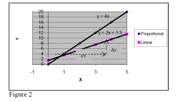
a constant and is called proportionality constant (4 in the case of figure).

In case of proportional relationships, if one of the quantities is multiplied by a factor, the other one is multiplied by the same factor, too.

(Ex. if X is increases 3 times, Y increases 3 times, too, because their ratio must remain unchanged, 4).

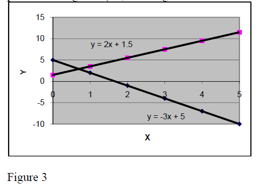
This is not true for linear relationships that are not proportional (verify for the linear relation in figure y = 2x + 1.5).

The general mathematical expression for linear relations is Y = a*X + b ...(1).

By coordinates of two points in data set one gets $Y_{1}=a*X_{1}+b\,\!$ and $Y_{2}=a*X_{2}+b\,\!$ ...(2)
Then, by subtracting the first equation from the second one $Y_{2}-Y_{1}\,\!$ = ΔY = $a*(X_{2}-X_{1})\,\!$ = a*ΔX

So, one gets that

ΔY = a*ΔX ...(3)

For all linear relations (proportional included), if the quantity X changes by ΔX the quantity Y changes by ΔY= a* ΔX .

Note: ΔY= $Y_{2}-Y_{1}\,\!$ not ΔY = $Y_{1}-Y_{2}\,\!$ (same for ΔX; see directions in fig1).

Note that a - coefficient is equal to the slope of straight line while b - coefficient is equal to the y value at the point where the straight line touches Y-axis.

The slope of a linear relation may be positive or negative (+2,+ 4 in fig.2 and +2 or –3 in fig.3).

In physics there are many linear and proportional relationships. Here are some of them:

Proportional:

Force to acceleration F = m*a

Elastic force to extension $F_{el}\,\!$ = k*Δx

Electric tension to current U = R*I

Linear:

Velocity to time $v=a*t+v_{0}\,\!$

Metal bars Length to temperature $l=c*T+l_{0}\,\!$

POWER FORM RELATIONSHIPS

If the experimental points are distributed around a line which slope changes from one to another region of X-values, one says that the relationship between quantities X and Y is described by a curve. In general, a curve can be fitted a power expressions. The following simpler forms are often met.

Parabolic relationship

$Y=a*X^{2}\,\!$ 

is widespread in different physics branches.

Example: We know that the acceleration of a object close to earth surface is $g=9.8m/s^{2}\,\!$ and if it is left to fall from rest at a given point O, the distance from O will increase in time as $y=a*t^{2}/2\,\!$. So, if one does experimental measurements of distance y at moment t and builds a graph, one will see a curved line.

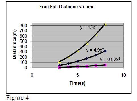
Then, comparing the ratios ($y/t^{2}\,\!$) one will find “almost the same value” a ~ 4.9 (= 9.8/2).
If one would repeat this experiment on Moon surface, one would get a ~ 0.82. On Jupiter surface one would get a ~ 13.
So, one may assert the following general physics’ law:

During the free fall, the distance of object from starting location increases in parabolic way with time. Note that the a- value depends on the planet.

Question: What is the gravitational acceleration on Moon and Jupiter surface (3rd curve)?…………………

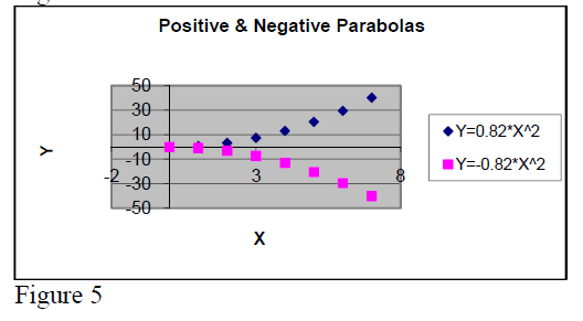
In dependence of the sign of the coefficient “a” one discerns positive and negative parabolas.
Their graph forms are presented in figure 4.

Note:

The general mathematical expression for a 

parabola is $y=a*x^{2}+b\,\!$. 

If b ≠ 0 the parabola top is not located at origin of coordinative system.

Inverse relationship

Y = const/X . 

This type of relationship must be considered when one of the measured quantities decreases while the other one increases. Verifying whether the product Y*X is almost constant for all measured data constitutes the first step trial.

If this is true one can confirm that the Y and X are related by an inverse relationship.

A physics experiment that would produce this kind of relationship: By compressing a gas its pressure P increases while its volume V decreases.

Another important inverse relationship in physics is the INVERSE SQUARE

Y = const / $X^{2}\,\!$. 

This is the mathematical form of gravitational and electrostatic forces F = const / $R^{2}$ exerted between two objects at distance R.

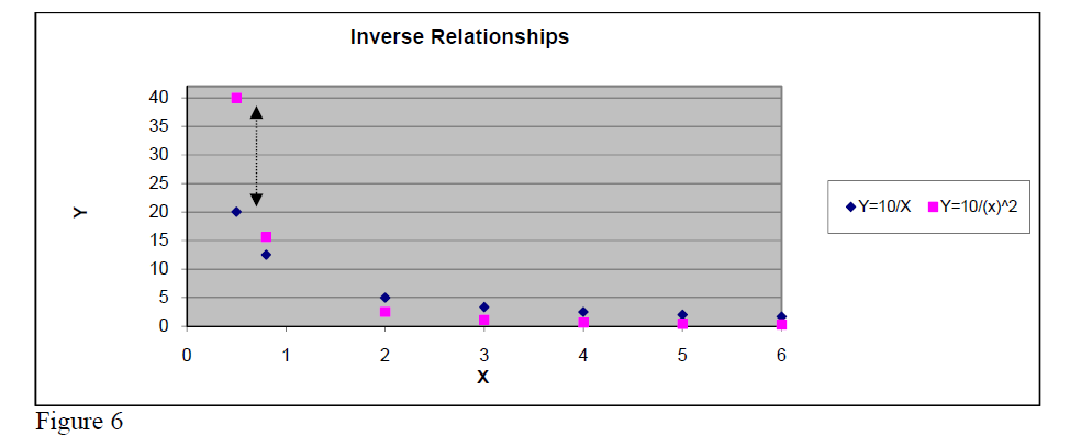
As shown in figure 6, the real difference between Inverse and Inverse Square relationships appears clearly only for small values of argument X.

So, when looking for the precise relationship one must compare X*Y to $X^{2}*Y\,\!$ for small values of X.

Exponential relationship

Y = a*Exp[$b*(X-c)^{d}\,\!$]. 

It is very common in physics. Its graph takes different forms in dependence on the values of parameters a, b, c, d.

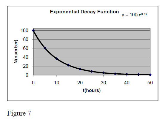
One very known example is that of radioactive nuclei which number decreases in time following the exponential expression N = $N_{0}\,\!$ Exp(−λ*t) . This expression is taken from the general one for a = $N_{0}\,\!$, b = -λ, X= t, c = 0 and d =1.





The figure 7 presents the graph of function

Y = 100 * Exp[−0.1*t]

FINDING THE ORDER OF MAGNITUDE OF THE CALCULATION RESULT

This is a kind of “estimation” on the size of the result within an order of (x10). One uses the approximations to get result estimations. It is very useful in answering questions like “find daily consumption of fruits in a city with 3 millions of habitants”. One starts by estimating say ~0.5kg fruits/day/person and follows $3*10^{6}*0.5=1.5*10^{6}\,\!$ i.e. essentially (as an order of magnitude) $10^{6}\,\!$ kg.

The basic technique for finding the order of magnitude requires approximating each of input numbers by the closest number containing only one significant figure and then performs the calculations.

Example: 2.135 + ${\frac {898.475*10.812}{7.891}}\,\!$ ≈ 2 + ${\frac {9*10^{2}*10^{1}}{8}}\,\!$ ≈ 2 + ${\frac {9*10^{3}}{8}}\,\!$ ≈ 1000

The precise answer is 1233.19 and it has the same order of magnitude (one thousand) as 1000.

Estimating first the order of magnitude many times prevent from small arithmetical mistakes. Say, if the normal step-by-step calculations give 12331.9 one sees quickly the existence of a mistake.